Usage

Plaxis connection

Along with padtest you will need to import plxscripting and connect with Plaxis following these instructions.

from plxscripting.easy import *
import padtest

password = "nicFgr^TtsFm~h~M"
localhostport_input = 10000
localhostport_output = 10001
s_i, g_i = new_server('localhost', localhostport_input, password=password)
s_o, g_o = new_server('localhost', localhostport_output, password=password)

WARNING

This code will not be repeated in every example, but it is assumed it was executed.

Create foundation model

WARNING

padtest employs units of kN and m by default.

The geometry of the foundation is given by:

d = 1.2 # Foundation depth
b = 2 # Foundation width
b1 = 0.5 # Foundation column width
d1 = 0.5 # Foundation width

Materials are defined by dictionaries containing the properties required in each case by Plaxis. Linear-Elastic, Mohr-Coulomb and Hardening Soil (HS) soil materials are supported. A Mohr-Coulomb material is used for the soil:

# Mohr-Coulomb soil material
soil = {}
soil['SoilModel'] = 'mohr-coulomb'
soil["DrainageType"] = 'Drained'
soil['gammaSat'] = 20 # kN/m3
soil['gammaUnsat'] = 17 # kN/m3
soil['e0'] = 0.2
soil['Eref'] = 4e4 # kN
soil['nu'] = 0.2
soil['cref'] = 0 # kPa
soil['phi'] = 35 # deg
soil['psi'] = 0 # deg

The foundation itself is modeled by plate elements. The concrete method generates the dictionary with the plate material properties from the desired compressive strength, unit weight and plate thickness.

# Plate material for a f'c=30MPa concrete slab with a 40cm thickness and 24kN/m3 unit weight
column = padtest.concrete(24, b1, fc=30)
# Plate material for a f'c=30MPa concrete slab with a 60cm thickness and 24kN/m3 unit weight
footing = padtest.concrete(24, d1, fc=30)

Create an axisymmetric foundation model using plate elements for the column and footing:

model = padtest.SPlate(s_i, g_i, g_o, b, d, soil, footing, column)

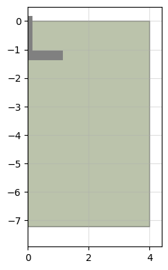
The resulting model geometry can be inspected visually in python:

model.plot(figsize=2.5)

Test

Static, failure, safety, dynamic loading and earthquake shake tests are available. A static load test is conducted using the load_test method. The test consist in consecutive load levels being applied to the foundation. Negative loads imply compression, while positive pull-out. Each load level is a phase where the load is set to the provided value.

testid = 'test A'
load = [-60, 0, -60] #kN
model.load_test(testid, load)

Calculation results are stored in a dataframe:

model.results

	test	phase	previous	plx id	previous plx id	location	step	time	sumMstage	SumMsf	...	M	qy0	qy1	qx	agx	agy	Fy target	Fx target	M target	ratchetting
0	None	construction	None	Phase_1	None	top	1.0	None	0.198850	None	...	0.0	0.0	0.0	0.0	0.0	0.0	0.000000	0.0	0.0	False
1	None	construction	None	Phase_1	None	top	2.0	None	0.397699	None	...	0.0	0.0	0.0	0.0	0.0	0.0	0.000000	0.0	0.0	False
2	None	construction	None	Phase_1	None	top	3.0	None	0.596549	None	...	0.0	0.0	0.0	0.0	0.0	0.0	0.000000	0.0	0.0	False
3	None	construction	None	Phase_1	None	top	4.0	None	0.994248	None	...	0.0	0.0	0.0	0.0	0.0	0.0	0.000000	0.0	0.0	False
4	None	construction	None	Phase_1	None	top	5.0	None	1.000000	None	...	0.0	0.0	0.0	0.0	0.0	0.0	0.000000	0.0	0.0	False
...	...	...	...	...	...	...	...	...	...	...	...	...	...	...	...	...	...	...	...	...	...
2257	test A	test A_stage_2	test A_stage_1	Phase_4	Phase_3	1.0	121.0	0.0	0.939505	1.0	...	0.0	0.0	0.0	0.0	0.0	0.0	-56.373698	0.0	0.0	False
2258	test A	test A_stage_2	test A_stage_1	Phase_4	Phase_3	1.0	122.0	0.0	0.953538	1.0	...	0.0	0.0	0.0	0.0	0.0	0.0	-57.214849	0.0	0.0	False
2259	test A	test A_stage_2	test A_stage_1	Phase_4	Phase_3	1.0	123.0	0.0	0.981585	1.0	...	0.0	0.0	0.0	0.0	0.0	0.0	-58.896135	0.0	0.0	False
2260	test A	test A_stage_2	test A_stage_1	Phase_4	Phase_3	1.0	124.0	0.0	0.991979	1.0	...	0.0	0.0	0.0	0.0	0.0	0.0	-59.519203	0.0	0.0	False
2261	test A	test A_stage_2	test A_stage_1	Phase_4	Phase_3	1.0	125.0	0.0	1.000000	1.0	...	0.0	0.0	0.0	0.0	0.0	0.0	-60.000000	0.0	0.0	False

2262 rows × 24 columns

By default 6 points are selected surveyed. The load application point at the surface, and points located at the foundation level at a distance of 0, 0.25, 0.5, 0.75 and 1 times b/2. The load test results can be inspected using the plot_test function.

model.plot_test('test A', location=0, legend=True)

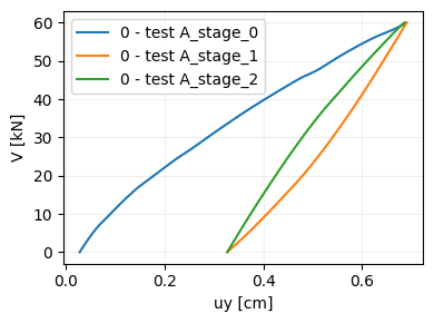
Multiple load tests can be performed in the same model.Each load test will start from the construction phase. **

Save/Load

Saving a model wipes out the Plaxis objects stored in it. This prevents the load test object from further communicating with Plaxis, so no additional can be performed. The information regarding the model geometry, material properties and test results is preserved.

model.save('exmaple_model.mdl')

WARNIGN: Saving the load test to memory whipes out the Plaxis objects. Test results and input parameters will still be avaiable, but no further interaction with Plaxis will be possible. The model can be restored with the <regen> method, but load tests will have to be recalculated to access the results whitin Plaxis.

 Do you whish to proceed: [Y/n]

The regen method regenerates the Plaxis model from a saved model so it can be used to calculate new tests. It can also recalculate the saved tests by setting the argument test to True.

model = padtest.load('exmaple_model.mdl')
model.regen(s_i, g_i, g_o, test=True)

General model settings

The model_type argument can be set to 'axisymmetry' (default) or 'planestrain'. Also, the title and comments of the model in Plaxis can be set with the title and comments arguments.

model = padtest.Plate(s_i, g_i, g_o, b, d, soil, footing, column,
                      model_type='planestrain', title='plane strain',
                      comments='This is a plane strain model example.')

Boundary conditions

The deformation_boundary_condition argument imposes user defined deformation boundary conditions to the model. A dictionary must be provided with some, or all, of the fields 'XMin', 'XMax', 'YMin' or 'YMax'. Supported values are "Free", "Normally fixed", "Horizontally fixed", "Vertically fixed" and "Fully fixed". If a boundary is not specified by the user, the default value is adopted.

The dynamic_boundary_condtions argument imposes user defined dynamic boundary conditions to the model to be used in a dynamic load test. A dictionary must be provided with some, or all, of the fields 'XMin', 'XMax', 'YMin' or 'YMax'. Supported values are "None" and "Viscous". If a boundary is not specified by the user, the default value is adopted.

The shake_boundary_condtions argument imposes user defined dynamic boundary conditions to the model to be used in a shake test. A dictionary must be provided with some, or all, of the fields 'XMin', 'XMax', 'YMin' or 'YMax'. Supported values are "None", "Viscous" and "Free-field". If a boundary is not specified by the user, the default value is adopted.

model = padtest.Plate(s_i, g_i, g_o, b, d, soil, footing, column,
                      deformation_boundary_condition={'XMin':'Fully fixed',
                                                      'YMax':'Horizontally fixed'},
                      dynamic_boundary_condtions={'XMin':'Viscous'})

Element type

The element_type argument controls the type of elements used in the model. It can be set to '6-Noded' or '15-Noded'. By default, 15-noded elements are used.

model = padtest.Plate(s_i, g_i, g_o, b, d, soil, footing, column,
                      element_type='6-Noded')

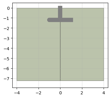
Preliminary model check

Waiting for Plaxis to build and run the initial phases can be time consuming only to check that the model has the correct geometry. The build attribute controls whether the Plaxis model gets build. By setting it to False the geometry can be inspecting with plot().

model = padtest.Plate(s_i, g_i, g_o, b, d, soil, footing, column, build=False)
model.plot()

The build() method creates the model in Plaxis so it can be used.

model.build()